Research Work
Physics:
1. Conducted a physics research project to measure the muon flux, muon lifetime, and measure the fermi coupling constant of Cosmic Ray Muons using the Muon Detector at Bellarmine University (Fall 2022 to Fall 2023):
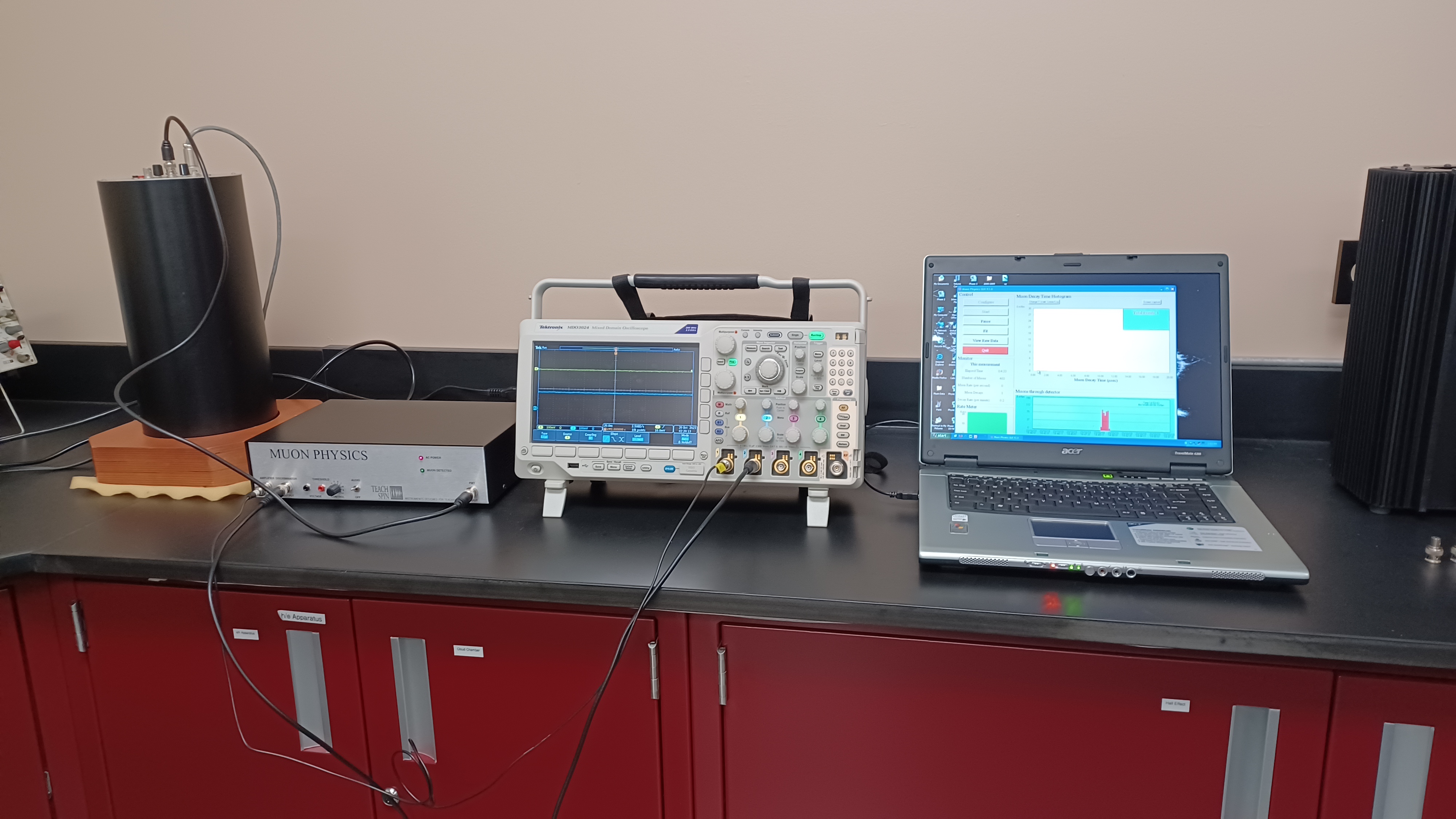
Muons produced from cosmic rays come to Earth from outer space, that originate outside the solar system from stellar/supernovae explosions in the Milky Way galaxy, called Galactic-Cosmic-Rays (GCRs). When primary cosmic rays (nuclei of hydrogen atoms. i.e. protons) traveling through the interstellar medium hit the Earth's atmosphere, they collide with the nuclei of the gas molecules, producing many secondary particles, including charged pions, that decay into a muon and two muon-neutrinos via the weak force. These cosmic ray muons travel about 99.8% of the speed of light, so their lifetime is time dilated, and hence can be detected on Earth using a muon detector. We used a desktop Cosmic Ray Muon Detector (CRMD) that contains cylindrical scintillator pads, a photomultiplier tube, and a high voltage power source, connected to an external data acquisition module via a BNC cable. The muon detector's data was fed to a laptop via a USB cable which ran the muon data acquisition software. This software displayed the muon hits, the number of muon decay events and the muon decay rate. As muons enter the muon detector, they decay into an electron, an electron neutrino and an anti-electron neutrino inside the plastic scintillator. The scintillator excitedly emits light that is detected by the photomultiplier tube, which produces a logic signal that triggers a timing clock. Several experimental runs were conducted to determine the mean muon flux, mean muon lifetime, and the Fermi Coupling constant which is a measure of the strength of the weak force.
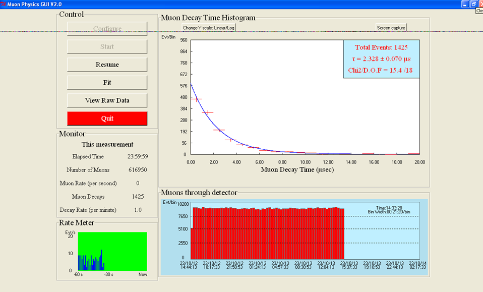
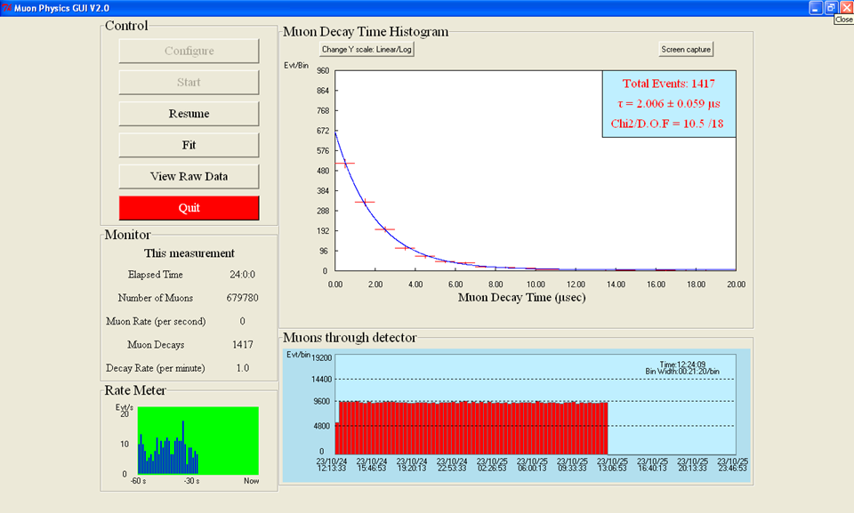
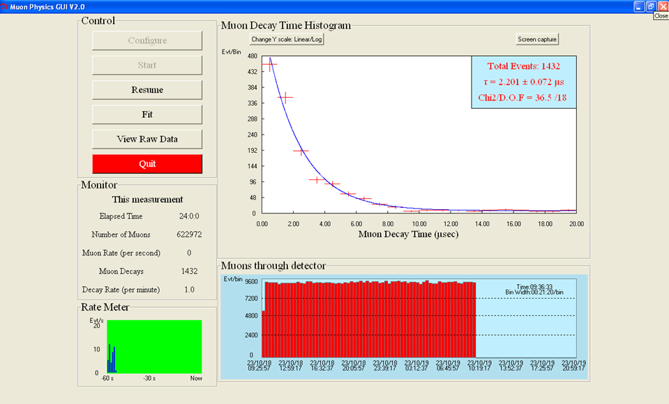
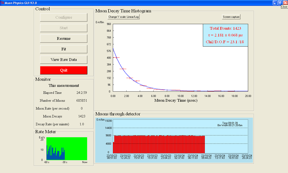
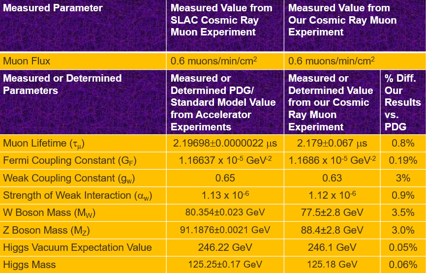
Based on the results obtained from our cosmic ray muon experiment, we can conclude that we can use cosmic ray muon data from a cosmic ray muon detector to successfully determine the properties of the Weak force that are comparable to results obtained from high energy particle accelerators. We were able to conclude that our data is comparable to the PDG values and is consistent with the Standard Model of Particle Physics. Cosmic ray muons are continuously entering Earth and therefore are continuously hitting us. Thus, knowing how many cosmic ray muons are hitting us at a given time may provide greater insight into its potential effects on the human body. One effect that may be of concern could be the potential radiation exposure from these muons. Based on our mean muon flux of 0.6 muon/min/cm2 we are able to determine that on average, about 5.4 trillion muons may hit an individual per year while about 500 trillion muons can hit an individual during their entire lifetime assuming they live for 90 years.
2. Analyzed NASA's exoplanet large datasets through data analysis, data filtering, and data visualization within Python to identify Earth-like exoplanets and determine the number of potentially habitable Earth like and Super-Earth like exoplanets orbiting a Sun like (type-G) star in the Milky Way galaxy's habitable zone (HZ) (Summer 2024 to Fall 2024):
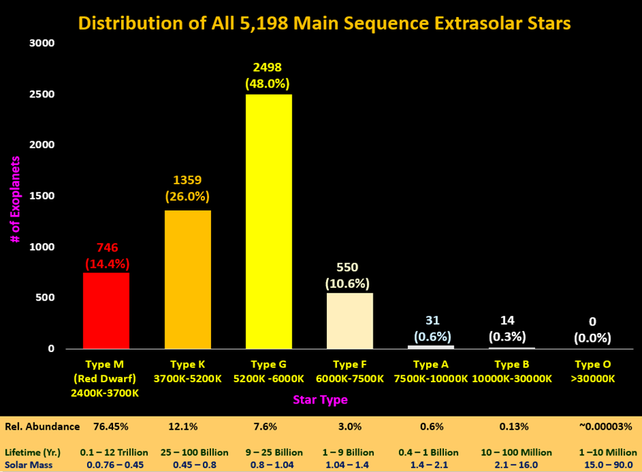
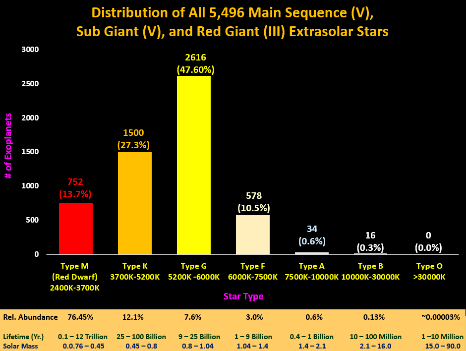
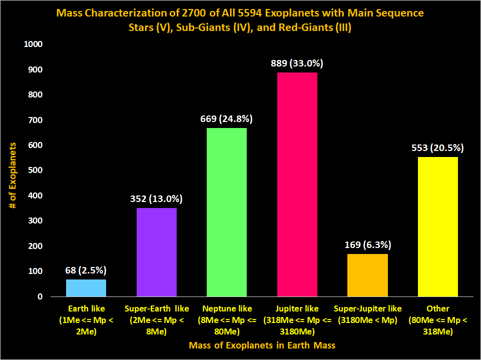
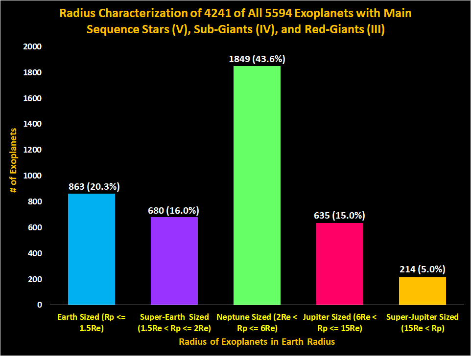
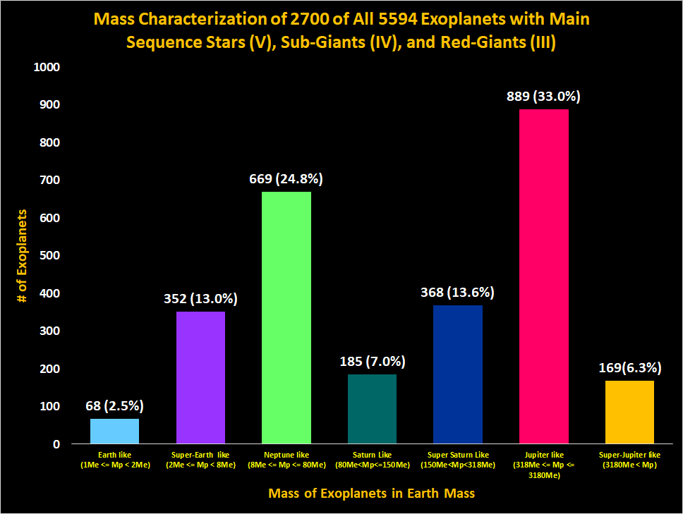
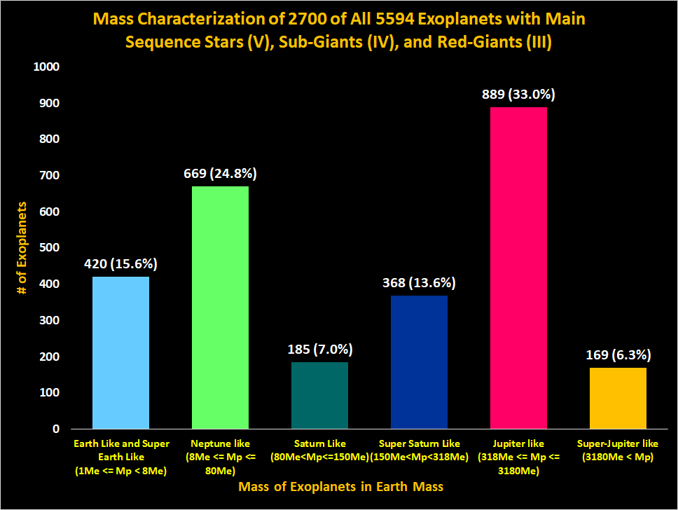
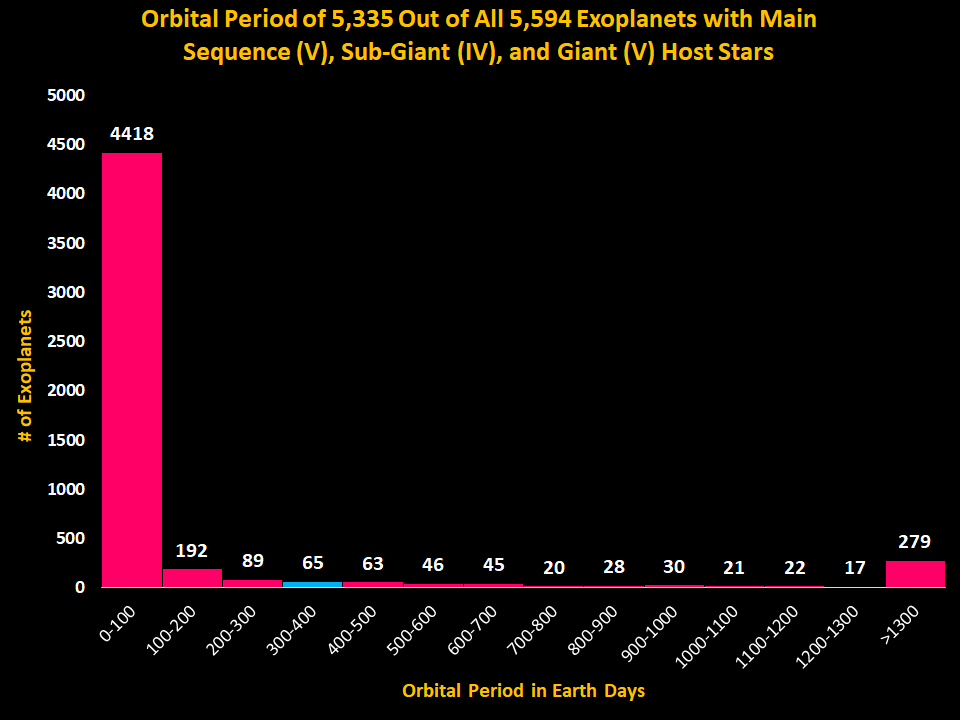
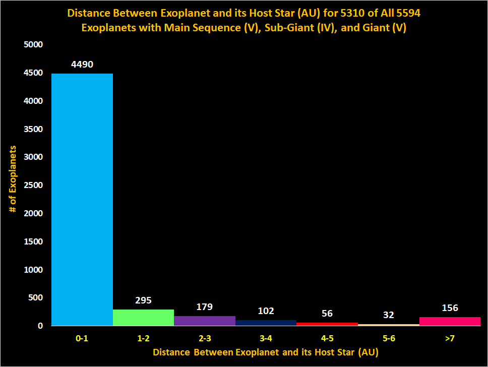
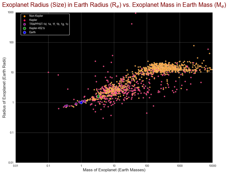
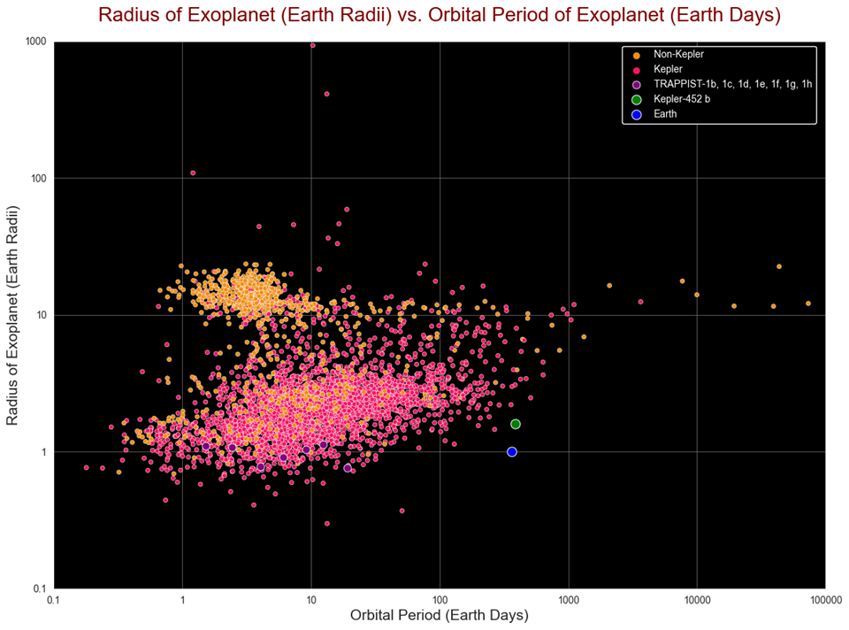
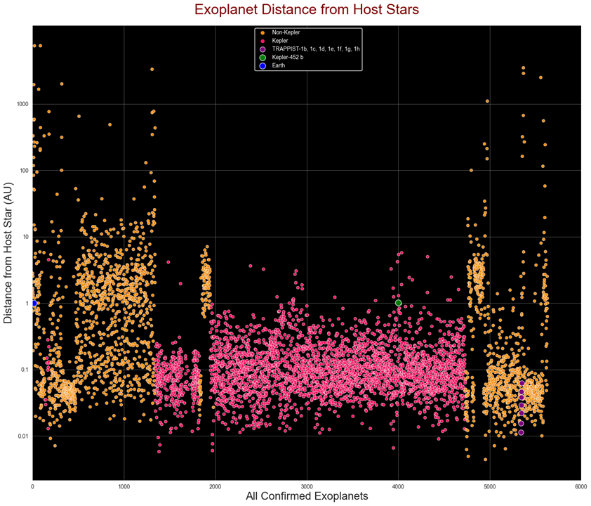
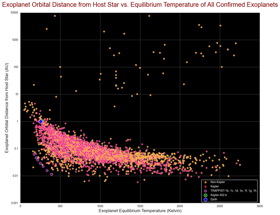
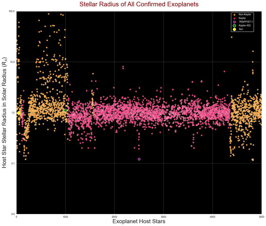
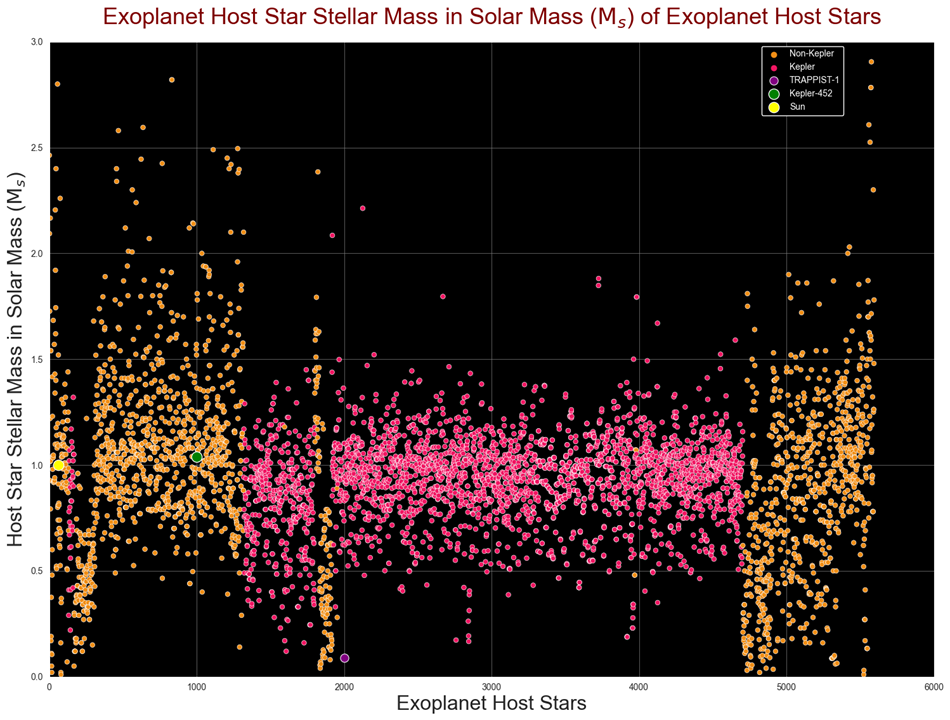
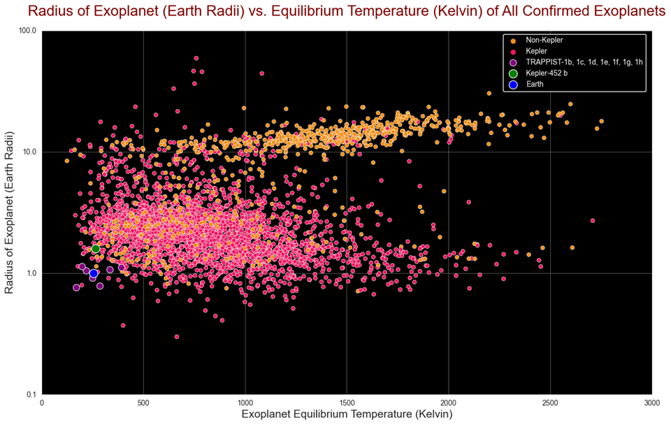
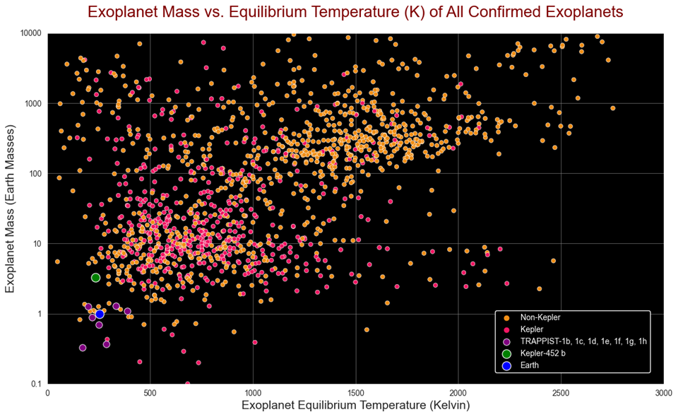
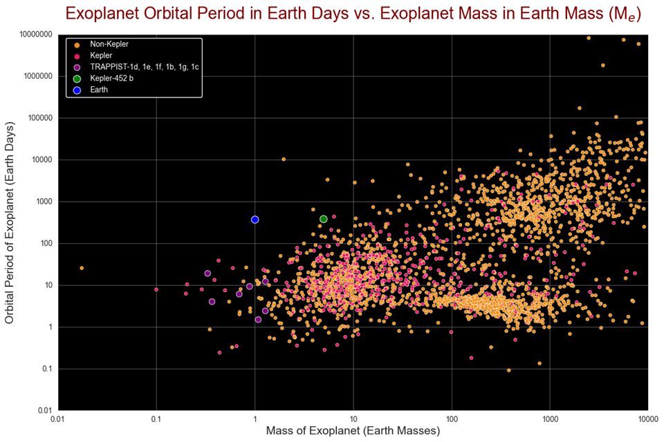
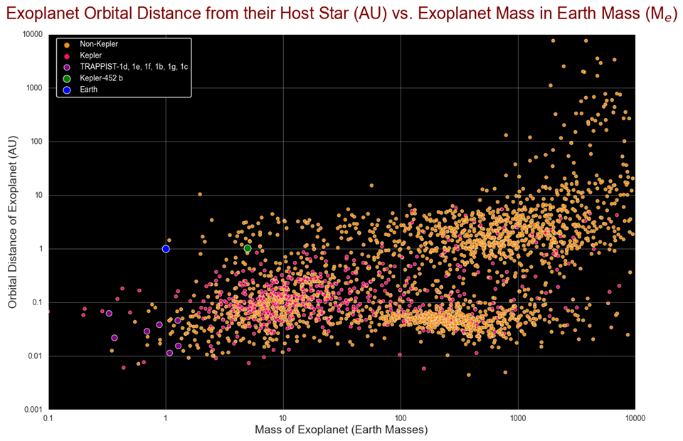
We have studied NASA's exoplanet large datasets (Big Data) that contains over one million data parameters of over 5600 exoplanets that have been discovered to date by both ground and space-based telescopes using various exoplanet detection methods and techniques. Using data analytics, we have extracted and filtered NASA's exoplanet dataset with codes written in Python to search for Earth-like exoplanets, we have named as Earth 2.0. We have also written visualization code in Python to plot several exoplanet parameters - such as exoplanet radii, mass, orbital period, surface temperature, exoplanets' distance from their host star, stellar type, stellar mass, stellar radius, and distance of exo-stars from Earth. We have also classified all the exoplanets into seven categories, based on a combination of their radius and mass as - Earth like, Super-Earth like, Neptune like, Saturn like, Super-Saturn like, Jupiter like, and Super-Jupiter like. Using data analytics and data visualization, we have made a prediction to determine the number of potentially habitable Earth like and Super-Earth like exoplanets orbiting a Sun like (type-G) star in our Milky Way galaxy's habitable zone (HZ).
All of the exoplanet data used in this research project was taken by various NASA missions. All Kepler exoplanet data was taken by NASA’s Kepler mission and the follow-up K2 mission. This also includes data from NASA’s Ecliptic Plane Input Catalog (EPIC) which is associated with the K2 mission as well data from NASA’s Kepler Object of Interest (KOI) catalog associated with the Kepler mission. This project utilized data of only confirmed exoplanets which orbited either a main sequence (V), sub-giant (IV), or red-giant (III) host star. Thus, data which was not a confirmed exoplanet was removed. Additionally, exoplanets which orbited anything other than a main sequence, sub giant, or red giant star were removed. This included exoplanets orbiting a binary star system, pulsar, white dwarf, brown dwarf, sub dwarf, Be star, etc. In the scatterplots, the pink dots display Kepler exoplanets while orange dots indicate Non-Kepler exoplanets. A habitable Earth-like rocky exoplanet Kepler-452b in our Milky Way galaxy is displayed with a large green dot. On each plot, Earth is displayed as a large blue dot. Purple dots display the exoplanets from the Trappist planetary system.
Prior to utilizing Python, we conducted pre-processing steps to remove unneeded columns, rename columns, and format the entries. The dataset contained numerous duplicate rows corresponding to a particular exoplanet. To reduce these duplicates into a single row, we used Python in Jupyter Notebook to impute the mean for numerical columns and mode for categorical columns for a given exoplanet. Prior to reducing the duplicate rows, we removed potential outliers to provide more accurate results by utilizing the z-score method. Through this, we flagged 25 entries in total as outliers. Out of which, we manually chose to keep 18 and removed 7 by comparing the difference between the means which included the outlier value and the means which did not include the outlier, if the difference was significantly larger, we chose to remove the given outlier.
Data Science:
1. Worked on a parallel computing research project to determine and analyze the performance of a 30-Node Raspberry Pi4 HTC (High Throughput Computing) Beowulf Cluster (Fall 2022):
At Bellarmine University, we have designed and built a Raspberry-Pi (RPi) cluster. A Beowulf cluster consists of one head node, and several client nodes connected together via a network switch. In a Beowulf cluster, all the nodes are dedicated to the cluster, and function as one system to process a job. The head node is the cluster’s console for compiling the source code and starting the parallel jobs. The server node controls the whole cluster and acts as the cluster’s head node for compiling the source code, starting parallel jobs. Each client node has a private IP address. All communication between the head node and client nodes and in between the client nodes are via the private IP addresses. In Parallel computing, the most important part of the implementation is the parallel code that runs on the cluster. Message Passing Interface (MPI) is a set of middleware functions that enable parallel programs to pass messages between processes of a parallel job.
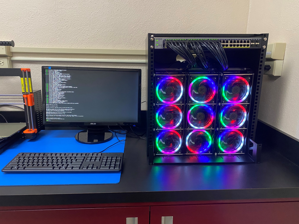
MPI is a collection of library routines that consists of a header file, a library of routines and a runtime environment that provides interaction/message-passing, and related operations between processors with a parallel system to enable parallel computation. The MPI code’s executable file after compilation must be able to spread itself across all the cluster’s nodes (usually done by running a script.) MPI can be used in Fortran, C and C++. Currently at least three widely used implementations of MPI exists: LAM/MPI, MPICH, and OpenMPI. OpenMPI is used by many TOP 500 Supercomputers. Open MPI is a high-performance, open-source middleware that is developed and maintained by a consortium of academic, research, and industry partners.
Not all applications will run effectively on a Beowulf Cluster. If a segment of a code takes less time to run than it takes to transmit it across all the other nodes of the cluster, executing that code segment serially on one node would be faster than using multiple nodes. The computation time of a parallel code depends on the time it takes to perform the communication between all the cluster nodes, which is called latency, i.e., communication overhead from the source (head node) to the destination (client nodes). Latency is a measure of delay. So, for lower computation time, due to latency, the speed up factor will vary, which is a difficult problem to deal with in cluster computing.
When latency is greater than the time it takes to run the code between all the nodes, the cluster computer will not be effective. This can happen in two different ways: One way is if the computation time is less, and the latency is greater than the time it takes to run the code across all the nodes, then you are better off running that code on fewer nodes. Another way is when you add too many nodes than that is necessary to run a parallel code, then the latency can become greater than the time it takes to run the code across all the nodes.
Instead of typing the commands one at a time manually on the keyboard to run jobs that can become cumbersome, Bash scripts can automatically run a job that can produce the output in a file. We wrote a Bash script for our parallel jobs. Scripts can be organized in such a way that it can generate the output data in an organized manner needed for data analyses. One of our goals was to test and explore the capabilities of the Raspberry-Pis to determine how well the Raspberry-Pis perform in a high-performance computing (HPC) environment for parallel processing tasks. The same set of MPI-based parallel codes and bash scripts that ran on our conventional Beowulf clusters were used on these Raspberry-Pi clusters.
We ran the following three MPI codes for our performance studies: Calculation Pi - The first MPI code calculates the value of Pi (p) up to 25 decimal places by integrating the function "4.0/( 1.0 + x2) "using n partitions (ranging from 100 million to 2 billions partitions), where n represents the number of partitions for the area under the integral. The MPI code also compares the result value of p with the known value of p and determines the error of the calculated value of p. Particle Simulation - The second MPI code randomly generates n number of simulated particles using the Monte Carlo method. Parallel Trapezoidal Method - The third MPI code uses the trapezoid method by integrating the function f(x) =1/x from a (100) to b (1000000) using n partitions ranging from 500 million to 5 billion.
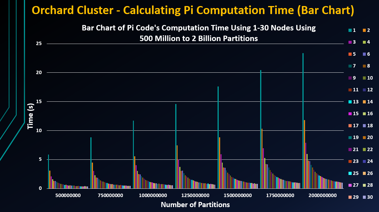
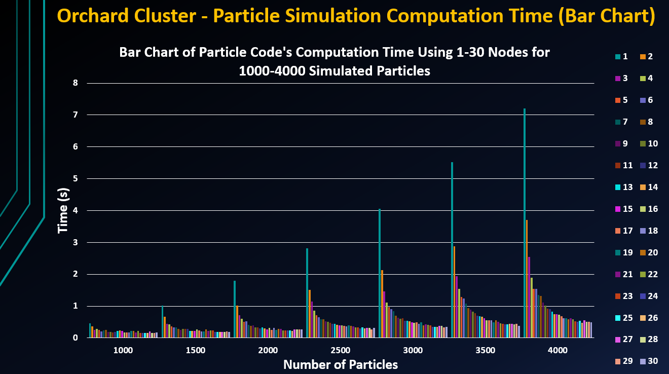
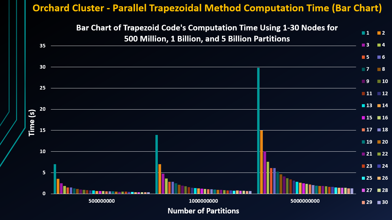
We looked at the speed-up factor which can be predicted by Amdahl’s law. Amdahl’s law gives the theoretical speed-up in latency of the execution of a task, given a fixed workload. Speed-up is a process for increasing performance between two systems processing the same problem. The speed up factor is found by the ratio of the Computation Time T1 for 1 Node over the Computation Time Tn for n Nodes.
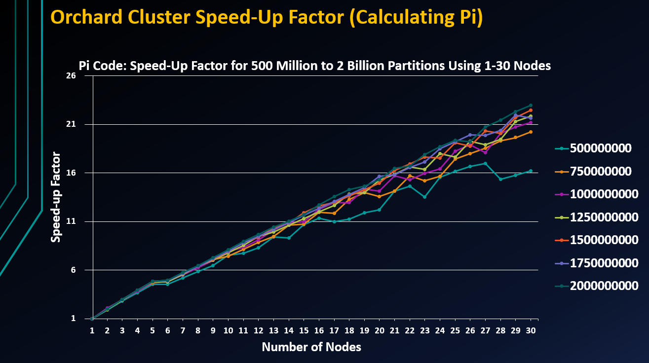
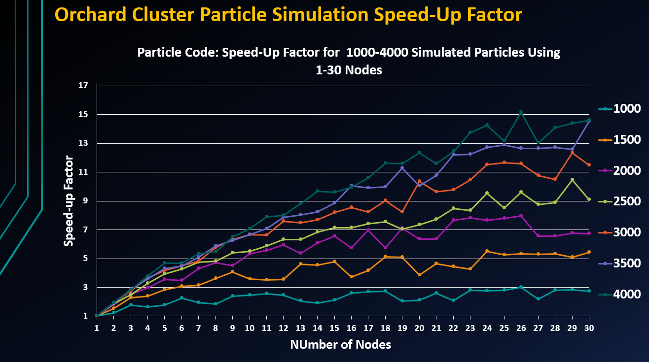
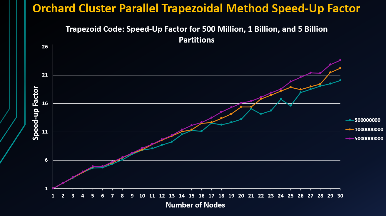
Reduction of the computation time of the parallel MPI codes can be achieved by spreading the computation across the nodes of the Raspberry Pi cluster. As expected, the results show the Computation time of both Raspberry Pi clusters dropped off exponentially as the # of nodes increased. For lower computation times, the effect of latency is evident, as expected. We noticed that that beyond 16 nodes, the reduction of computation time is very nominal for both clusters. Depending on the MPI code for lower computation times, due to latency, the speed up factor varied, as expected. In accordance with Amdahl’s law, the Speed Up Factor increased linearly for the more CPU intensive jobs with higher computation time for all three MPI codes. The expected performance gain of the Raspberry Pi4 processor (Orchard cluster) is about 14 times that of the Raspberry Pi1 processor (Vine cluster) but based on the computation time data, the actual performance gain after 4 nodes decreases due to latency for lower computation time. So, the actual computation time will be greater than the expected computation time and hence the actual performance gain will be lower than the expected performance gain. In this project, we have showed that Raspberry-Pi technology can be used to build cost-effective low-powered high-performance, table-top Raspberry-Pi clusters to conduct computational tasks. Whereas a 120-core conventional HPC rack-mount cluster would cost over $85,000 to build (that needs AC cooling), our 120-core HPC Raspberry-Pi Orchard cluster with comparable capabilities only costs $8,500 to build (i.e. ten times less) that only needs fans for cooling (no AC) and much less physical space.
2. Developed software called Object-Brightness Analyzer for Rubin Observatory (OBARO) in Python using the Gaussian Model Mixture Model machine learning algorithm to detect the brightness of all astronomical objects from the Rubin Observatory's PhoSim (Photon Simulation) and Data Preview (DP0.2) simulation data sets (Summer 2024 to Fall 2024):
We have developed and written a software called Object-Brightness Analyzer for Rubin Observatory (OBARO) in Python using the Gaussian Model Mixture (GMM) machine learning(ML) algorithm that can automatically detect and calculate the brightness of all astronomical objects from the PhoSim Rubin (LSST)-Survey-#1 simulation data sets and from Rubin Observatory's Data Preview (DP0.2) simulation data sets. The PhoSim Rubin(LSST)-Survey-#1 data sets were generated using Bellarmine University's Tier2 Grid Supercomputer that is linked to the Open Science Grid (OSG) cyberinfrastructure. The OBARO software uses statistical analysis and machine learning to plough through and scan all the astronomical objects and calculate the mean pixel value, mean pixel value error, surface brightness, surface brightness error, area, pixel count for both the object and its background as well as the flux and magnitude for the astronomical object. Once the OBARO software runs all the FITS files, it will produce an output file in XML format for analysis. The OBARO software can run on a PC/laptop. We will present the results of brightness studies of astronomical objects in some of the PhoSim Rubin (LSST) Simulated Survey #1 data sets using Phosim versions 5.1.7 and 5.3.23 and in some of the Data Preview 0.2 data sets.
Light emmited from astronomical objects from outer space known as photons get distorted due to gravitional lensing and the atmosphere. Then there is a refraction and scattering of light due to the LSST telescope itself. There are also detector effects which all play a crucial role in the process of photons entering the LSST telescope's camera. The photons travel through a cylindrical column of the atmosphere. As the photons enter through the three mirrors of the telscope, they bounce off the primary mirror and into the secondary mirror before reflecting backwards from the tertiary mirror and into the focal plane of the telscope's camera lens. The photons are then converted into photo-electrons as they drift to the CCD readout panels which evntually produce an image. We used Photon Simulator or PhoSim which is a simulation tool that can produce realistic simulated LSST images. It turns out that significant fraction of all measurement systematics with LSST will come from the complex physical effects of the atmosphere, telescope, and camera that distort the light from astrophysical objects.
Photon Simulator (PhoSim) is a simulation tool that can produce realistic simulated LSST images. These images are simulated at a single location on the sky coering 10 1q. Deg. PhoSim simulates 10 billion photons per CCD at a rate of 500,000 photons/s and generates sky images by simulating the path of photons through the atmosphere, LSST’s 3 mirrors, and 3 camera lens with the camera’s physical effects to determine the propagation of light to the focal plane using a photon-based Monte Carlo approach. PhoSim uses fast ray‐trace algorithms. PhoSim uses FFTs (Fast Fourier Transforms) and fast intercept calculations to determine a comprehensive physical description of the atmosphere, LSST telescope and CCD camera in order to simulate realistic optical/IR/X-ray images. Phosim uses hydrodynamic-based descriptions of atmospheric turbulence, elasticity theory calculations of optical deformations, and electrostatic simulations of sensors.
The distortion of light will be imprinted in the LSST images, and therefore the most robust way understanding the systematics is through these high-fidelity PhoSim image simulations using Monte-Carlo techniques. PhoSim can predict all the primary and secondary image properties from physical models of the atmosphere and the telescope parameters. All physical effects for optical light that determine the shapes, locations, and brightness of individual stars and galaxies can be accurately represented using PhoSim. PhoSim generates the images by collecting photons and converting them into pixels. PhoSim can be used to perform detailed astronomical measurement systematic studies for advanced image processing and machine learning algorithms.
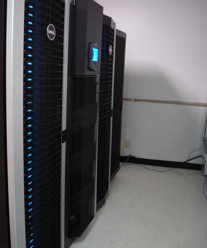
We have a dedicated Tier2 OSG (Open Science Grid) site at Bellarmine University which ran Phosim and generated the PhoSim Rubin (LSST)-Survey-#1 data sets. PhoSim Rubin (LSST)-Survey-#1 data sets are stored a Bellarmine University. Currently, Kentucky's only OSG site is at Bellarmine University. Our Tier2 supercomputer has 408 cores, 1300GB of RAM and 375TB of storage space. The PhoSim Rubin (LSST) Simulated Survey #1 5.1.7 data set was saved as tar files. Each seed# contains 3024 individual 1 Mpixel images, that constitute one full LSST focal plane image, totaling 3.024 Gpixels for all 3024 image segments. It took us about 1 week to run PhoSim for each seed since each seed contained 3024 FITS files. We also have a copy of the entire DP0 data sets stored on our Tier2 OSG supercomputer.
In the Run-1 simulation data set, each seed# is a new MC run. There are 35 MC runs (seed1000 to seed1034) for PhoSim version 5.1.7, and 8 MC runs (seed1000 to seed1007) for PhoSim version 5.2.23. Currently we are process of running PhoSim version 5.4.10. The simulation run time for each seed# with 3024 readout chip segments varies- anywhere from 1 day to 5 days, on average. The PhoSim Rubin (LSST) Simulated Survey #1 datasets contains over 140,000 simulated images at a single location on the sky covering 10 square degrees using all of the atmosphere, telescope, and sensor physics of PhoSim v5.1 to v5.4.
3024 individual CCD readout segments are collaged together to form a full LSST focal plane image of 3.024 Gigapixels (3024 Megapixels). The 3024 individual 1 Mpixel images are generated in segments according to the numbering of the LSST camera’s focal plane’s 189 CCDs in the 21 science rafts. Each PhoSim seed# contains a collage of the 16 readout CCD chip segments for each 3x3 CCD arrays (S00, S01, S03, S10, S11, S12, S20, S21, S22).
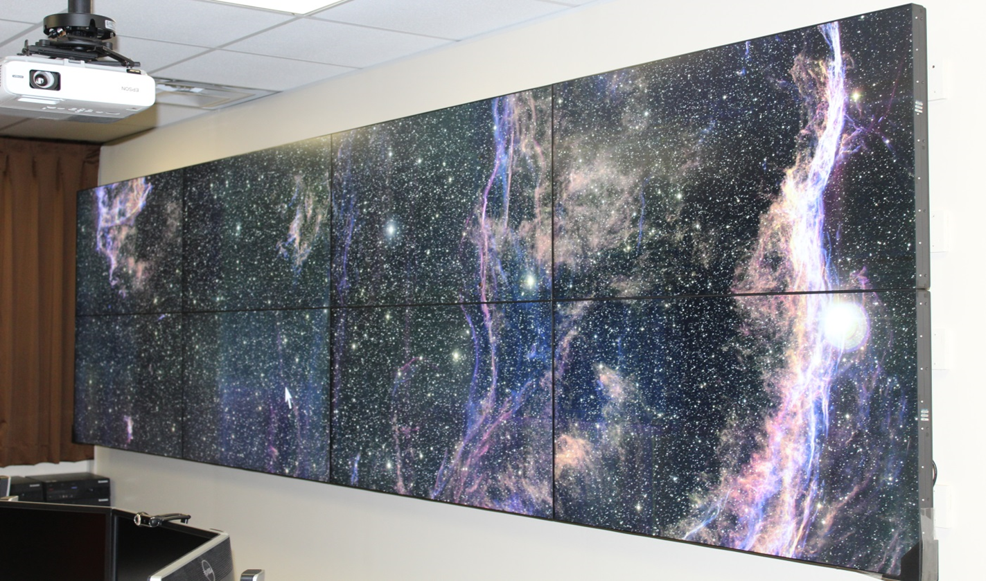
For this research project, we utilized our Hyperwall Visualization System at Bellarmine University which displayed the FITS file images. Our visualization system is comprised of a 8-Tiled Display Wall in a 4x2 tiled format which are 6 Feet Wide x 4.5 Feet High (8 HD 55” TVs) where [(4×1920 (2K) pixels) × (2×1080 (1K) pixels) = 7680 (8K) pixels × 2160 (2K) pixels = 16.5 MPixels. The image below shows a Supernova Remnant (SNR) Displayed on the Hiperwall Visualization System.
Robotics
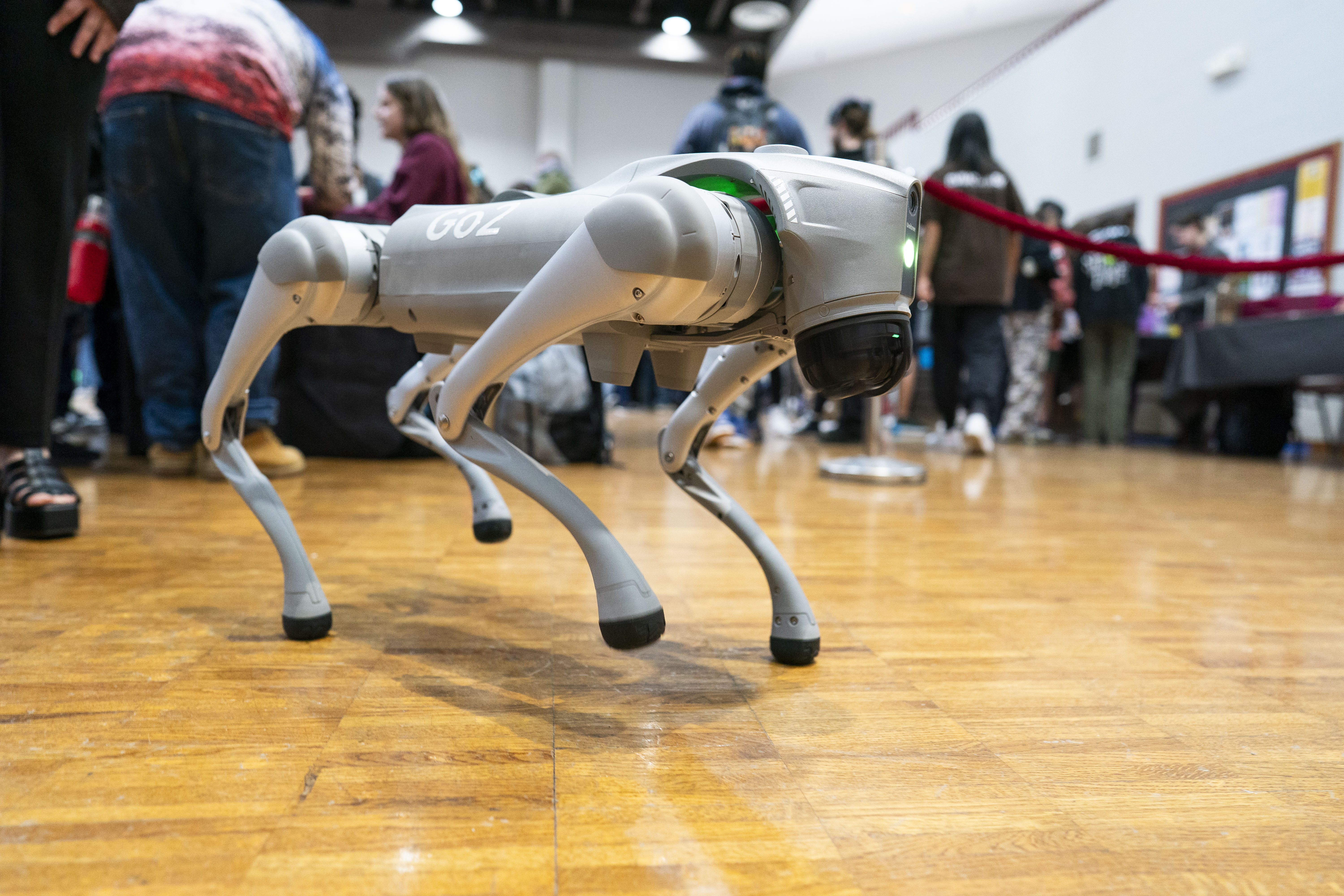
1. Programming the Unitree Go2 Robotic Dog nicknamed "Rover" to perform various movements and tasks:
I programmed the Unitree Go2 Robotic Dog to crouch, sit, jump forward, stretch, and shake hands. Additionally, we utilizing voice activation to allow the robotic dog to listen and respond to certain voice commands. This includes word responses to voice commands to "shake hand," "lie down," "stand up," and "roll over."
STEM Education
In 2022 Bellarmine University received funding from the National Science Foundation (NSF) for the Noyce Track-1 project - Recruiting, Preparing, and Supporting Highly Qualified Kentucky Science and Mathematics Teachers. The Noyce Knights Scholars Program (NKSP) at Bellarmine Univeristy aims to prepare, support and certify 25 highly qualified diverse middle school science and high school Physics, Chemistry, Biology, and Mathematics teachers.
This Noyce Track-1 project builds on the Bellarmine University’s NSF funded Noyce Capacity Building project (2019 – 2021) that strengthened the STEM teacher education infrastructure, by forming new partnerships, and recruitment pipelines. Upon certification (based on the teaching certification), all NKSP scholars will be placed at a JCPS (Jefferson County Public Schools) or another high-need school district’s middle/high school (upon request) or at an Archdiocese of Louisville Catholic middle/high school (upon request). The Noyce Knights Scholars Program (NKSP) colaborates with the Kentucky Science Center (KSC), Univeristy of Kentucky, Kentucky Community & Technical College System (KCTCS), and the JCPS STEM Academies.
We had three cohort of Noyce summer interns at the Kentucky Science Center (KSC) as part of the Noyce Knights Program (NKSP). Cohort 1 internship was held in summer 2019 that was supported by our earlier Noyce Capacity Building grant. Cohort 2 and Cohort 3 internship were held in summer 2023 and 2024, respectively, that was supported by the Noyce Track-1 grant.
I conducted the data analysis to evaluate performance trends across multiple cohorts, identifying key patterns and insights. In addition, I developed a custom visualization software in Python called "Viz Plot", designed to graphically represent complex data. This software enhanced the clarity and accessibility of performance metrics, enabling more effective communication of results to both technical and non-technical audiences.
Particle Physics
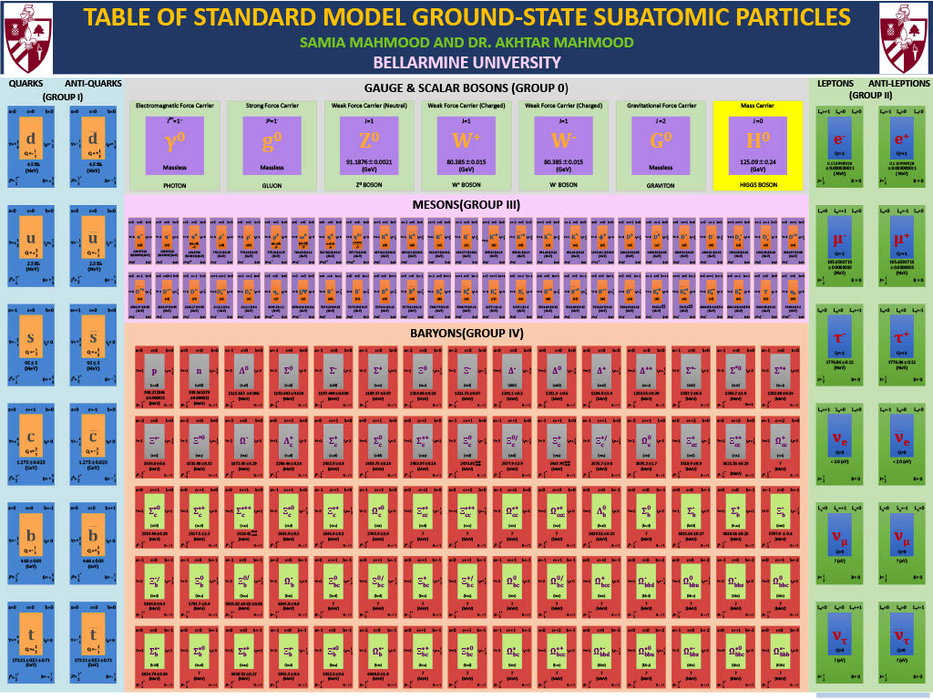
I worked on a research project to develop a table of all the possible ground-state Standard Model subatomic particles - quarks, leptons, mesons, baryons and the force-carrier particles, including the Higgs Boson with all quantum properties - Mass (if measured), Lifetime (if measured), Spin, Total Angular Momentum, Parity, Charge-Conjugation, Isospin, Hypercharge, Baryon, and Lepton number (L). This table of Standard Model ground-state subatomic particles will be like the periodic table of elements which can be hung next to the periodic table of elements in Physics classrooms and labs.
High Energy Physics
I am currently engaged in a research project focused on the search for a hypothetical Z′ (Z-prime) boson using a subset of data collected by the ATLAS detector at the Large Hadron Collider (LHC). This study targets the dilepton decay channels, specifically the electron–positron and muon–antimuon final states, which provide clean experimental signatures and high sensitivity to potential new neutral gauge bosons beyond the Standard Model. The analysis is conducted using the Hypatia and Camelia frameworks to reconstruct events, apply selection criteria, and study invariant mass distributions in search of deviations from Standard Model expectations.
A central component of my work is the development and integration of automated analysis pipelines, aimed at improving efficiency, reproducibility, and scalability across large datasets. By incorporating automation into event selection, background estimation, and visualization, this project seeks to streamline the analysis workflow while maintaining rigorous statistical and experimental standards.